
Cluster Post 2 | Module 4: Data Analysis and Presenting Results
From Concept to Submission Series | 2026
Descriptive Statistics: What to Report and How to Read Them
The module overview defines mean, median, mode, standard deviation, and range. This post goes deeper: which measure of central tendency is appropriate for which type of data, how to read a distribution before running any inferential tests, what skewness and kurtosis tell you and why they matter, and how to build a descriptive statistics table that gives readers everything they need to evaluate your data.
Descriptive Statistics Are Not Optional Preliminaries
Many researchers treat descriptive statistics as a formality — a table of means and standard deviations to present before the real analysis. This misunderstands their function. Descriptives are not summaries of your data; they are your first look at what your data actually is, and they determine whether the inferential analyses that follow are appropriate.
Every inferential test assumes something about the distribution of your data. t-tests and ANOVA assume approximate normality. Correlation and regression assume linearity and homoscedasticity. If you run these tests without first examining whether their assumptions are plausible, you are working blind — your significance tests may be invalid, and you will not know.
A distribution that looks skewed in your descriptives tells you to check normality formally before running parametric tests. A mean that is dramatically different from the median signals outliers that may be influential. A standard deviation so large that it implies negative values on a scale with a floor of zero tells you your data is not behaving as you expected. Descriptive statistics reveal these problems before they corrupt your analysis.
Which Measure of Central Tendency to Use
The choice of mean, median, or mode is not arbitrary — it depends on the level of measurement and the shape of the distribution. Using the wrong measure produces a misleading summary of your data.
The mean: powerful but sensitive
The mean is the most informative measure of central tendency when data is approximately normally distributed and measured at interval or ratio level. It uses every data point and is mathematically tractable — it is the basis for most parametric statistics.
Its sensitivity to outliers is its main limitation. A set of incomes in a village where most households earn ₹20,000–₹40,000 per month but one household earns ₹2,000,000 will have a mean far above what any typical household earns. The mean describes no one’s actual situation. This is why income, wealth, and similarly skewed distributions are almost always reported with medians, not means.
The median: robust but less powerful
The median is the appropriate measure when data is skewed, when outliers are present and meaningful (not errors), or when the data is at ordinal level. It is less sensitive to extreme values and provides a better description of the typical case in non-normal distributions.
For Likert-scale data — the 1-to-5 or 1-to-7 response scales common in social science surveys — there is ongoing methodological debate about whether to report means or medians. Strictly, Likert items are ordinal (the distance between 2 and 3 may not equal the distance between 4 and 5), which would argue for medians. In practice, treating Likert scale composites as interval and reporting means is widely accepted when the composite is made up of multiple items and the distribution is approximately symmetric. For single Likert items, medians and frequency distributions are more appropriate.
The mode: for categorical data
The mode is the appropriate summary for nominal (categorical) data where means and medians are meaningless — you cannot compute the average gender or the median course of study. Report the mode alongside frequency counts and percentages for categorical variables.
| Variable type | Appropriate central tendency measure |
| Nominal (gender, college, subject) | Mode + frequency (%) |
| Ordinal — single Likert item | Median + frequency distribution |
| Ordinal — multi-item Likert composite scale | Mean + SD (if approximately symmetric) |
| Interval / ratio — normally distributed | Mean + SD |
| Interval / ratio — skewed or with outliers | Median + IQR (interquartile range) |
Understanding Distribution Shape: Skewness and Kurtosis
Mean and standard deviation tell you the centre and spread of your distribution. Skewness and kurtosis tell you about its shape — information that is essential for deciding whether parametric tests are appropriate.
Skewness
A perfectly symmetric distribution has skewness = 0. Positive skewness (right skew) means the distribution has a long tail to the right — most values are low, with a few very high values pulling the mean upward. Negative skewness (left skew) means the tail extends to the left.
Rule of thumb: skewness values between -1 and +1 are generally considered acceptable for parametric analysis. Values between -2 and +2 are sometimes acceptable depending on sample size (larger samples are more robust to modest skewness). Values beyond ±2 warrant concern and should be addressed — either through transformation (log, square root) or by using non-parametric tests.
Common skewed distributions in social science research: — Income and wealth: strongly positive skew — Response times: positive skew (most are fast, some very slow) — Years of education in general population samples: negative skew (floor effect at zero, most people complete at least primary) — Test scores in competitive examinations: often negative skew (most participants score high, few very low)
Kurtosis
Kurtosis describes the height of the peak and the thickness of the tails. A normal distribution has kurtosis = 3 (or excess kurtosis = 0 in software that subtracts 3). Leptokurtic distributions (positive excess kurtosis) have a high peak and heavy tails — more extreme values than a normal distribution. Platykurtic distributions (negative excess kurtosis) are flatter with thinner tails.
Heavy-tailed distributions (high positive kurtosis) are particularly problematic for statistical tests because they produce more extreme outliers than the normal distribution assumes. If your kurtosis exceeds ±3 (excess), treat your distribution with suspicion and check for outliers before proceeding with parametric analysis.
The Standard Deviation: Reading It Correctly
The standard deviation (SD) tells you the typical distance of individual data points from the mean. This is more informative than the range, which is determined entirely by the two most extreme values and tells you nothing about where most of the data sits.
A useful check: the mean ± 2 SD should cover approximately 95% of your data if the distribution is normal. If your mean is 50 and your SD is 30, then approximately 95% of values should fall between -10 and 110. But your scale only goes from 0 to 100. A value of -10 is impossible. This tells you the distribution is not normal — it is probably skewed or bounded in a way that makes the SD a misleading summary of spread. Report the median and interquartile range instead.
When comparing SDs across groups or variables, consider them relative to the mean — the coefficient of variation (SD / mean × 100) expresses variability as a percentage of the mean and allows comparisons across scales with different units or ranges. A SD of 15 means something very different on a scale from 1 to 100 than on a scale from 1 to 7.
Outliers: When to Keep Them and When to Address Them
An outlier is a data point that is unusually far from the rest of the distribution. The critical question is whether it is unusual because it is a data entry error, because it genuinely represents an extreme case that exists in the population, or because the distribution is skewed in a way that produces legitimate extreme values.
These three possibilities require different responses. An entry error should be corrected or removed. A genuine extreme case may need to be retained — removing it would distort your picture of the population. A distribution that routinely produces extreme values may need to be transformed or analysed with non-parametric methods.
The standard detection approaches
- Z-score threshold: Values with |z| > 3.29 are conventionally flagged as outliers (p < .001 in both tails). Compute z-scores for each variable and examine any cases beyond this threshold.
- IQR method: Values below Q1 – 1.5×IQR or above Q3 + 1.5×IQR are flagged. This is the method used by box plots and is less sensitive to the distributional assumptions of the z-score approach.
- Visual inspection: Histograms, box plots, and Q-Q plots reveal outliers and distributional anomalies that summary statistics can miss. Run these before any inferential analysis.
Report what you found and what you did about it. “Three cases were identified as outliers (z > 3.29) on the anxiety variable. Examination of original survey responses confirmed these were valid responses, not entry errors. Analyses were conducted with and without these cases; results did not differ substantively, so the full sample was retained.” This is the level of transparency reviewers expect.
Building the Descriptive Statistics Table
The descriptive statistics table is typically the first table in the results section. Its purpose is to give readers a complete picture of your variables before they encounter any inferential results. A well-constructed descriptive table means readers do not need to ask “what were the typical values?” or “how variable was the data?” while reading your results.
For interval and ratio variables, report: N (sample size for that variable, not the whole study), mean, standard deviation, minimum, maximum, and skewness. For ordinal variables with distributions that matter, add the median and IQR. For nominal variables, report frequency counts and percentages in a separate table or in the text.
Descriptive statistics table entry (APA format): Variable: Peer_contact_frequency N: 442 M: 3.41 SD: 1.87 Min: 0 Max: 12 Skew: 0.84 Reading this: The typical student had peer mentor contact approximately 3.4 times per month (SD = 1.87). The range from 0 to 12 and the positive skew (0.84) suggest that while most students had low to moderate contact, a smaller group had frequent contact. The skewness is within the acceptable range for parametric analysis but warrants checking for normality before proceeding.
Always include your N for each variable, not just the overall sample size. If fifteen participants skipped the peer contact question, the N for that variable is 427, not 442. A reader who does not know this cannot properly evaluate your results.
🔱 For Law Students
Descriptive statistics appear in legal research wherever quantitative variables are analysed — sentencing studies, case duration analysis, compliance rate research, judicial decision studies. The principles above apply directly, with two additional considerations specific to legal data.
Interpreting descriptive statistics on legal outcomes
Legal outcome variables — case duration, sentence length, bail amounts, compensation awards — are almost always positively skewed. Cases that resolve quickly cluster at low values; a small number of highly complex or repeatedly adjourned cases produce a long right tail. This means the mean duration is almost always higher than the median, and the mean alone gives a misleading picture of what is typical.
Always report medians alongside means for skewed legal variables, and always provide the distribution shape to contextualise the summary statistics. A statement that “the mean case duration in Special POCSO Courts was 847 days (SD = 412)” without noting the positive skew (which implies most cases resolved faster) is technically accurate but practically misleading.
Frequency distributions for categorical legal variables
Many legal variables are categorical: case type, court level, outcome, bench composition, geographic jurisdiction. These require frequency distributions and percentages, not means. A table showing that 62% of bail applications were granted, 31% were refused, and 7% were disposed of on other grounds tells a reader more than any single summary statistic would.
When comparing frequencies across categories — for example, grant rates across different courts or different types of offences — also report the absolute numbers alongside percentages. A grant rate of 75% based on 4 cases is very different from a 75% grant rate based on 400 cases, and readers need both pieces of information to evaluate the finding.
References
- Field, A. (2024). Discovering Statistics Using IBM SPSS Statistics (6th ed.). Sage.
- Tabachnick, B. G., & Fidell, L. S. (2022). Using Multivariate Statistics (8th ed.). Pearson.
- Creswell, J. W., & Creswell, J. D. (2022). Research Design: Qualitative, Quantitative, and Mixed Methods Approaches (6th ed.). Sage.
- American Psychological Association. (2020). Publication Manual of the APA (7th ed.).
- Frost, J. (2023). Regression Analysis: An Intuitive Guide. Statistics By Jim Publishing. statisticsbyjim.com
Next: Cluster Post 3 — Inferential Statistics: Choosing and Reporting the Right Test

10 Structural Mistakes That Get Research Papers Rejected — And How to Fix Every One
Cluster Post 7 | Module 1: Understanding the Structure of Research Papers and Theses From…

Academic Tone: From Principles to Practice
Cluster Post 3 | Module 5: Organising Chapters, Maintaining Academic Tone, and Preparing Submission-Ready Documents…

Academic Writing Mastery: The Complete 2026 Guide to Research Papers & Thesis Writing
Academic Writing Mastery Your research deserves to be read. This complete guide transforms your ideas…
Citation Styles Explained: APA, MLA, Chicago, IEEE, and Bluebook
Cluster Post 4 | Module 2: The Academic Writing Process From Concept to Submission Series …

Complete Thesis Structure: A Chapter-by-Chapter Guide
Cluster Post 6 | Module 1: Understanding the Structure of Research Papers and Theses From…
Data Analysis and Results Presentation: Complete Guide for Quantitative, Qualitative & Legal Research (2026)
Data Analysis and Results Presentation: Why Data Analysis Determines Research Credibility Here’s what separates published…
Descriptive Statistics: What to Report and How to Read Them
Cluster Post 2 | Module 4: Data Analysis and Presenting Results From Concept to Submission…
Formatting Thesis for Institutional Submission
Cluster Post 4 | Module 5: Thesis Writing and Submission From Concept to Submission Series …

How to Start Writing — and Keep Going
Cluster Post 1 | Module 2: The Academic Writing Process From Concept to Submission Series …

How to Write a Methods Section That Reviewers Will Trust
Cluster Post 3 | Module 1: Understanding the Structure of Research Papers and Theses From…

How to Write a Research Introduction That Reviewers Cannot Ignore
Cluster Post 2 | Module 1: Understanding the Structure of Research Papers and Theses From…

How to Write Clear Engaging Academic Prose
Cluster Post 2 | Module 2: The Academic Writing Process From Concept to Submission Series …
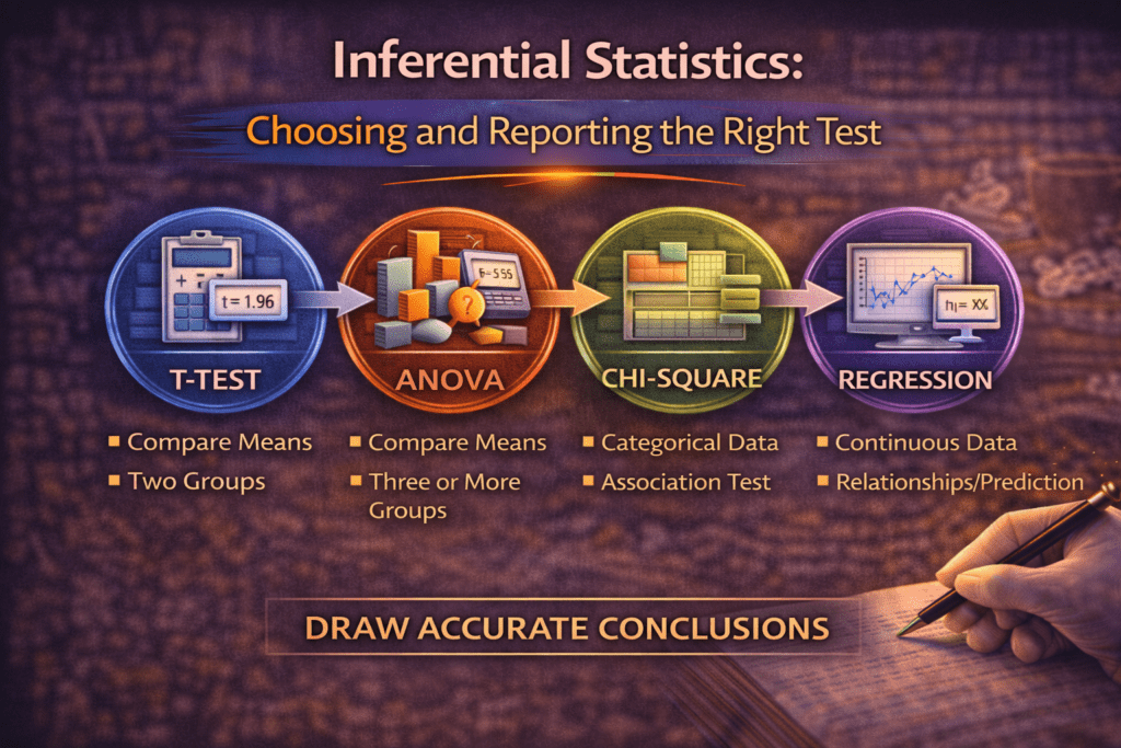
Inferential Statistics: Choosing and Reporting the Right Test
Cluster Post 3 | Module 4: Data Analysis and Presenting Results From Concept to Submission…
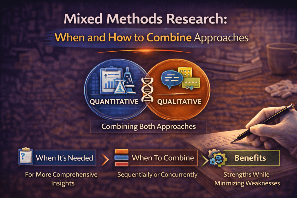
Mixed Methods Research: When and How to Combine Approaches
Cluster Post 5 | Module 3: Research Methodologies From Concept to Submission Series | 2026…

Organization and Academic Tone: Complete Guide to Professional Scholarly Writing (2026)
Why Organization and Academic Tone Matter More Than You Think Here’s what thesis examiners notice…
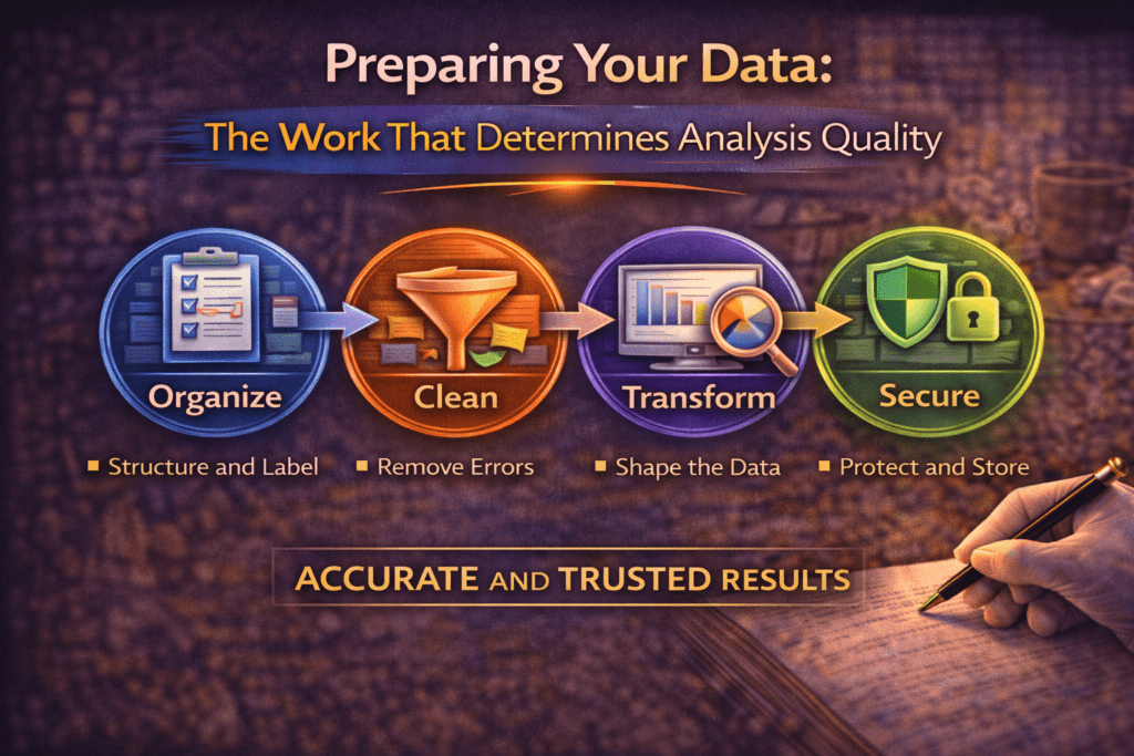
Preparing Your Data: The Work That Determines Analysis Quality
Cluster Post 1 | Module 4: Data Analysis and Presenting Results From Concept to Submission…
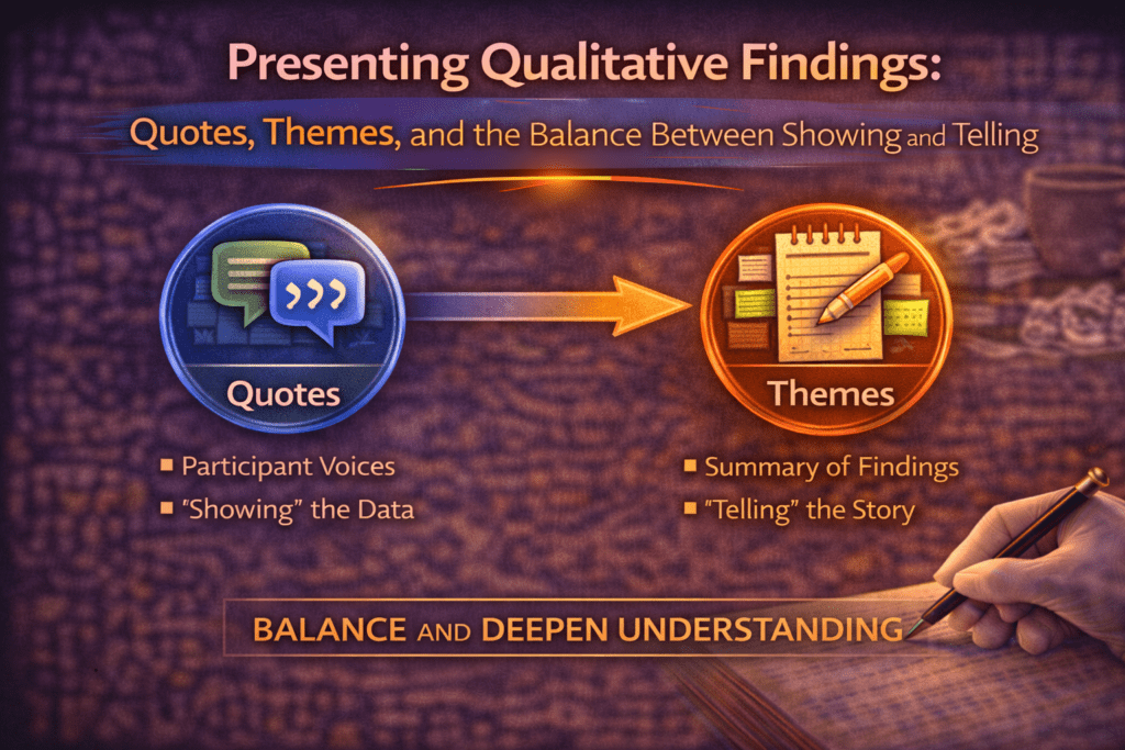
Presenting Qualitative Findings: Quotes, Themes, and the Balance Between Showing and Telling
Cluster Post 5 | Module 4: Data Analysis and Presenting Results From Concept to Submission…
Qualitative Data Collection and Analysis: Interviews, Coding, and Trustworthiness
Cluster Post 4 | Module 3: Research Methodologies From Concept to Submission Series | 2026…
Qualitative Research Design: Choosing the Right Approach
Cluster Post 3 | Module 3: Research Methodologies From Concept to Submission Series | 2026…
Quantitative Research Design: From Hypothesis to Valid Results
Cluster Post 2 | Module 3: Research Methodologies From Concept to Submission Series | 2026…

Reference Management: Zotero and Mendeley from Setup to Submission
Cluster Post 5 | Module 2: The Academic Writing Process From Concept to Submission Series …
Research Ethics in Practice: What Ethics Forms Don’t Tell You
Cluster Post 7 | Module 3: Research Methodologies From Concept to Submission Series | 2026…
Research Methodologies: Complete Guide to Quantitative, Qualitative, Mixed Methods & Legal Research (2026)
Why Methodology Determines Research Quality Here’s what thesis examiners focus on first: your methodology section…

Research Paradigms: Why Your Philosophical Stance Shapes Everything
Cluster Post 1 | Module 3: Research Methodologies From Concept to Submission Series | 2026 ←…
Sampling: Choosing Who to Study and How Many
Cluster Post 6 | Module 3: Research Methodologies From Concept to Submission Series | 2026…
Statistical Assumptions: The Checks Most Researchers Skip
Cluster Post 4 | Module 4: Data Analysis and Presenting Results From Concept to Submission…

The Academic Writing Process: Complete Guide from First Draft to Submission (2026)
From Concept to Submission: A Complete Guide to Research Paper and Thesis Writing Module 2,…

The Complete Guide to Research Paper Structure: IMRAD Format, Thesis Organization & Academic Writing (2026)
From Concept to Submission: A Complete Guide to Research Paper and Thesis Writing Module 1:…
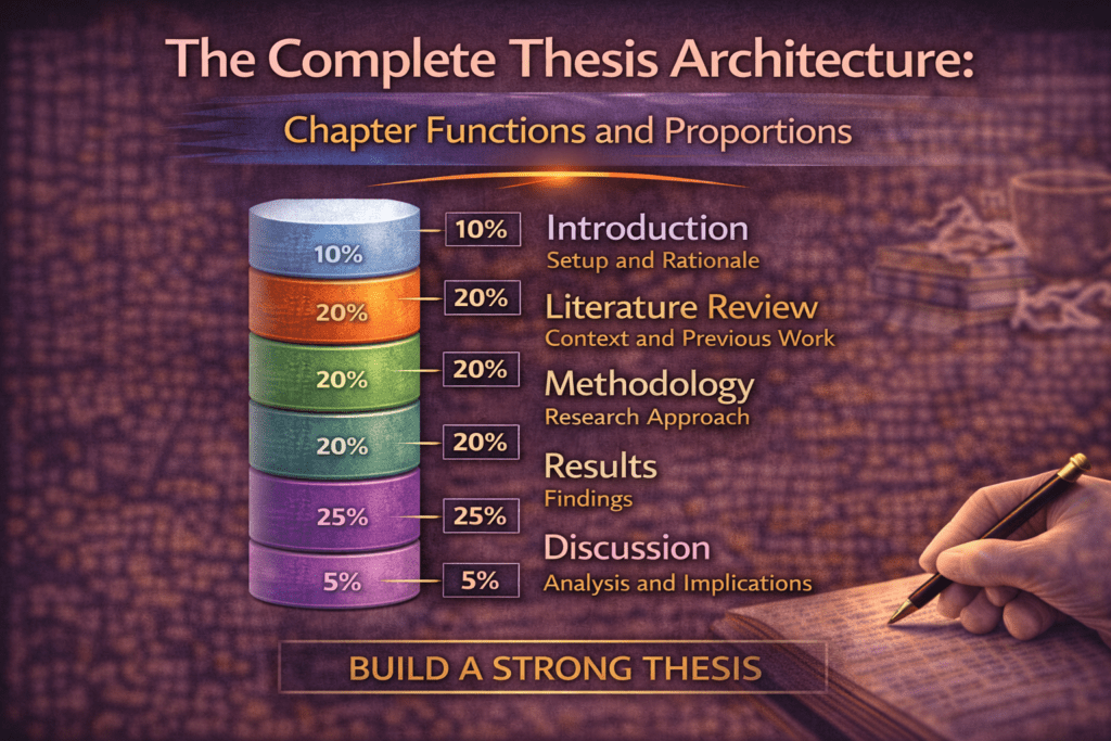
The Complete Thesis Architecture: Chapter Functions and Proportions
Cluster Post 1 | Module 5: Organising Chapters, Maintaining Academic Tone, and Preparing Submission-Ready Documents…
The Discussion Section: How to Turn Findings Into Knowledge
Cluster Post 5 | Module 1: Understanding the Structure of Research Papers and Theses From…