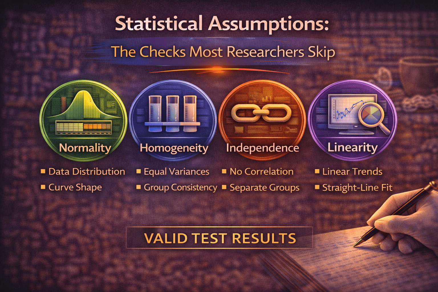
Cluster Post 4 | Module 4: Data Analysis and Presenting Results
From Concept to Submission Series | 2026

Statistical Assumptions: The Checks Most Researchers Skip
The module overview mentions that statistical tests have assumptions but does not explain them. This post covers: exactly what each major assumption requires, how to test it, what the consequences of violation are, and what to do when an assumption is violated — so you can check assumptions systematically rather than hoping your data happens to meet them.
Why Assumptions Matter
Every parametric statistical test is derived mathematically under specific conditions about the data. When those conditions are met, the test performs as advertised: the p-values are accurate, the confidence intervals are correctly calibrated, and the Type I error rate is what you specified. When conditions are violated, all of this breaks down — sometimes subtly, sometimes severely.
Assumption violations do not always produce obviously wrong results. A t-test run on moderately non-normal data with a reasonable sample size may produce a p-value very close to the correct one. But a t-test run on severely skewed data with a small sample may produce a p-value that is dramatically incorrect — meaning your conclusion about significance may be wrong, and you will not know unless you checked.
The standard practice is: check assumptions before running inferential tests, report what you found, and report what you did when violations were detected. Reviewers and examiners expect this. A methodology section that says “a t-test was conducted” without any mention of assumption checking signals either that the checks were not done or that the researcher does not know they should be done.
Normality
Normality is the assumption that the data — or in many cases, the residuals from the analysis — are drawn from a normally distributed population. It is required by t-tests, ANOVA, Pearson correlation, and linear regression (for regression, it is the residuals that must be normal, not the raw data).
How to test it
- Visual inspection: Histograms with a normal curve overlay, Q-Q plots (quantile-quantile plots), and box plots. A Q-Q plot shows each data point’s quantile against the quantile expected under normality — points that fall close to the diagonal line indicate normality; systematic deviation indicates departure.
- Shapiro-Wilk test (for N < 50): A formal significance test of normality. A non-significant result (p > .05) indicates the data are not significantly different from normal. The limitation: with large samples, even trivial departures from normality become significant, making the test misleading for large datasets.
- Skewness and kurtosis: As covered in Cluster Post 2, values outside ±2 for skewness and ±3 for excess kurtosis warrant concern.
What to do when normality is violated
- With large samples (N > 100): Parametric tests are generally robust to moderate normality violations by the central limit theorem — sampling distributions of means tend toward normality as N increases. Proceed with parametric tests but note the violation.
- With small samples and severe violations: Use the non-parametric equivalent: Mann-Whitney U instead of independent t-test, Wilcoxon signed-rank instead of paired t-test, Kruskal-Wallis instead of one-way ANOVA, Spearman’s rho instead of Pearson correlation.
- Transformation: Log, square root, or inverse transformations can normalise positively skewed distributions. Apply the transformation to the variable before analysis. Report the transformation in your methodology and interpret results in terms of the transformed variable.
Reporting example when normality is violated: “Examination of histograms and Q-Q plots, combined with Shapiro-Wilk tests (ps < .05 for both groups), indicated that peer contact frequency scores were positively skewed in both conditions. Given the small sample sizes (n = 28 and n = 31), Mann-Whitney U tests were conducted rather than independent t-tests.”
Homogeneity of Variance
Independent samples t-tests and one-way ANOVA assume that the variance in the outcome variable is approximately equal across groups being compared. When group variances are substantially different, the test’s ability to control the Type I error rate is compromised.
How to test it
Levene’s test is the standard check, available in SPSS and most statistical software alongside the t-test and ANOVA output. A significant Levene’s test (p < .05) indicates that variances differ significantly across groups.
What to do when violated
- For independent t-tests: Use Welch’s t-test (also called the unequal variances t-test), which adjusts degrees of freedom to account for unequal variances. SPSS reports this automatically alongside the standard t-test. Report Welch’s version when Levene’s test is significant.
- For ANOVA: Use Welch’s ANOVA or the Brown-Forsythe F. Both are available in SPSS under the “Robust tests of equality of means” option. For post-hoc tests when variances are unequal, use Games-Howell rather than Tukey’s HSD.
Reporting example: “Levene’s test indicated that the assumption of homogeneity of variance was violated, F(2, 437) = 8.14, p < .001. Welch’s ANOVA was therefore used, F(2, 211.3) = 11.87, p < .001. Post-hoc comparisons were conducted using the Games-Howell procedure.”
Independence of Observations
All standard parametric tests assume that each observation is independent of every other — that knowing one participant’s score tells you nothing about another’s. This assumption is violated when participants are nested within groups (students within classrooms, patients within hospitals, employees within organisations), when the same participant provides multiple observations (repeated measures), or when participants influence each other’s responses.
Independence violation is the most consequential assumption violation and the one most often ignored. When observations are not independent — for example, when students from the same classroom are more similar to each other than to students from other classrooms — standard errors are underestimated, t-values and F-values are inflated, and p-values are too small. This is a systematic bias that cannot be corrected after the fact by changing the analysis.
Detecting and addressing violations
- Clustered data: If participants are sampled from intact groups (schools, colleges, wards), use multilevel modelling (also called hierarchical linear modelling or mixed models) to account for the clustering. If multilevel modelling is not feasible, at minimum report the intraclass correlation (ICC) — the proportion of variance that lies between clusters — and acknowledge its implications.
- Repeated measures: Use repeated measures ANOVA or mixed models that explicitly model the within-person correlation. Do not treat repeated measures from the same participant as independent observations in a standard ANOVA.
- Matched pairs: Use paired rather than independent t-tests when the same participant provides pre-test and post-test data, or when participants have been matched.
Linearity and Homoscedasticity in Regression
Linear regression assumes that the relationship between each predictor and the outcome is linear, and that the variance of the residuals is constant across all levels of the predictors (homoscedasticity). Both assumptions are checked through residual plots.
How to check
After running a regression, produce a scatterplot of the standardised residuals (y-axis) against the standardised predicted values (x-axis). In software: SPSS calls this ZRESID vs. ZPRED; R produces it as the first plot in plot(model).
- Linearity: The residuals should show no systematic pattern. A curved pattern (U-shape or inverted U) indicates non-linearity — the relationship between predictor and outcome is not linear. Consider transforming the predictor or adding a quadratic term.
- Homoscedasticity: The spread of residuals should be roughly constant across the range of predicted values (a random scatter around zero). A fan shape — residuals spreading out as predicted values increase — indicates heteroscedasticity. Use heteroscedasticity-robust standard errors (available in R, Stata, and with add-ons in SPSS).
Multicollinearity in multiple regression
When predictor variables are highly correlated with each other, regression coefficients become unstable and hard to interpret. This is multicollinearity, and it is a specific concern in multiple regression with several related predictors.
Check the Variance Inflation Factor (VIF) for each predictor. VIF values above 5 indicate moderate multicollinearity; values above 10 indicate severe multicollinearity requiring action. Solutions include removing one of the correlated predictors, combining them into a composite, or using regularised regression methods such as ridge regression.
A Systematic Assumption-Checking Workflow
| Test | Check before running |
| Independent t-test | 1. Normality of DV in each group (histogram, Q-Q plot, Shapiro-Wilk if N < 50) 2. Homogeneity of variance (Levene’s test) 3. Independence of observations |
| One-way ANOVA | Same as t-test, applied to each group separately |
| Pearson correlation | 1. Normality of both variables 2. Linearity of relationship (scatterplot) 3. No extreme bivariate outliers |
| Multiple regression | 1. Linearity (residual vs. predicted plot) 2. Normality of residuals (Q-Q plot of residuals) 3. Homoscedasticity (residual vs. predicted plot) 4. Independence of residuals (Durbin-Watson for time-series data) 5. Multicollinearity (VIF for each predictor) |
| Chi-square | 1. Expected cell frequencies ≥ 5 (if not, use Fisher’s exact test) 2. Independence of observations |
Build this workflow into your analysis routine. Run descriptives and assumption checks first, every time, before touching the inferential tests. The fifteen minutes this takes is insurance against discovering an unchecked violation after your results section is written.
For Law Students
Statistical assumption checking in empirical legal research follows the same principles as social science research. Two contexts arise frequently in Indian legal research that warrant specific attention.
Clustered court data and the independence assumption
Studies using multiple cases from the same court, judge, or district violate the independence assumption. Cases heard by the same judge are not independent — they share the judge’s interpretive tendencies, workload pressures, and procedural preferences. Cases from the same district share local legal culture, infrastructure quality, and bar composition.
Ignoring clustering in legal outcome data produces artificially small standard errors — the same problem described above for nested social science data. If your dataset includes cases from multiple courts or multiple judges, report the intraclass correlation at the court and judge level, and consider multilevel models that account for this nesting. At minimum, acknowledge the limitation and note that your standard errors may be conservative estimates of the true uncertainty.
Non-normality is the default for legal outcome variables
As noted in Cluster Post 2, legal outcome variables — sentence length, case duration, compensation amounts, bail quantum — are almost always non-normal. Do not check normality hoping to confirm it; check it expecting to find violation and plan your analysis accordingly. Non-parametric tests or data transformations should be considered the default starting point for continuous legal outcome variables, with parametric tests used only when the normality check confirms approximate normality after transformation.
References
- Field, A. (2024). Discovering Statistics Using IBM SPSS Statistics (6th ed.). Sage.
- Tabachnick, B. G., & Fidell, L. S. (2022). Using Multivariate Statistics (8th ed.). Pearson.
- Gelman, A., & Hill, J. (2007). Data Analysis Using Regression and Multilevel/Hierarchical Models. Cambridge University Press.
- Hayes, A. F. (2022). Introduction to Mediation, Moderation, and Conditional Process Analysis (3rd ed.). Guilford Press.
- Frost, J. Statistical assumption testing resources. statisticsbyjim.com
Next: Cluster Post 5 — Presenting Qualitative Findings: Quotes, Themes, and the Balance Between Showing and Telling

The Complete Guide to Research Paper Structure: IMRAD Format, Thesis Organization & Academic Writing (2026)
From Concept to Submission: A Complete Guide to Research Paper and Thesis Writing Module 1:…
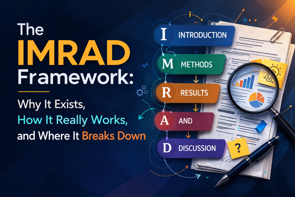
The IMRAD Framework: Why It Exists, How It Really Works, and Where It Breaks Down
Cluster Post 1 | Module 1: Understanding the Structure of Research Papers and Theses From…

How to Write a Research Introduction That Reviewers Cannot Ignore
Cluster Post 2 | Module 1: Understanding the Structure of Research Papers and Theses From…

How to Write a Methods Section That Reviewers Will Trust
Cluster Post 3 | Module 1: Understanding the Structure of Research Papers and Theses From…
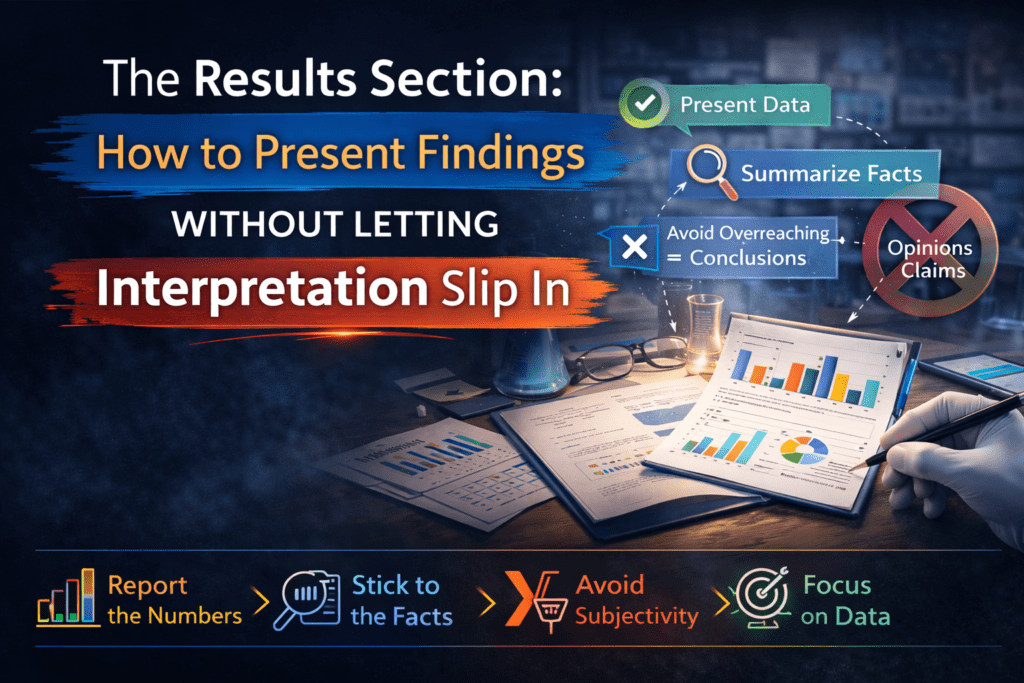
The Results Section: How to Present Findings Without Letting Interpretation Slip In
Cluster Post 4 | Module 1: Understanding the Structure of Research Papers and Theses From…

The Discussion Section: How to Turn Findings Into Knowledge
Cluster Post 5 | Module 1: Understanding the Structure of Research Papers and Theses From…

Complete Thesis Structure: A Chapter-by-Chapter Guide
Cluster Post 6 | Module 1: Understanding the Structure of Research Papers and Theses From…

10 Structural Mistakes That Get Research Papers Rejected — And How to Fix Every One
Cluster Post 7 | Module 1: Understanding the Structure of Research Papers and Theses From…

The Academic Writing Process: Complete Guide from First Draft to Submission (2026)
From Concept to Submission: A Complete Guide to Research Paper and Thesis Writing Module 2,…

How to Start Writing — and Keep Going
Cluster Post 1 | Module 2: The Academic Writing Process From Concept to Submission Series …

How to Write Clear Engaging Academic Prose
Cluster Post 2 | Module 2: The Academic Writing Process From Concept to Submission Series …
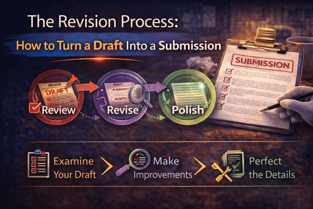
The Revision Process: How to Turn a Draft Into a Submission
Cluster Post 3 | Module 2: The Academic Writing Process From Concept to Submission Series …

Citation Styles Explained: APA, MLA, Chicago, IEEE, and Bluebook
Cluster Post 4 | Module 2: The Academic Writing Process From Concept to Submission Series …

Reference Management: Zotero and Mendeley from Setup to Submission
Cluster Post 5 | Module 2: The Academic Writing Process From Concept to Submission Series …
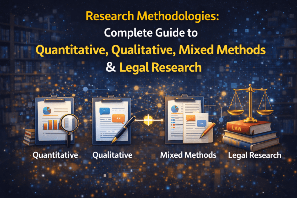
Research Methodologies: Complete Guide to Quantitative, Qualitative, Mixed Methods & Legal Research (2026)
Why Methodology Determines Research Quality Here’s what thesis examiners focus on first: your methodology section…

Research Paradigms: Why Your Philosophical Stance Shapes Everything
Cluster Post 1 | Module 3: Research Methodologies From Concept to Submission Series | 2026 ←…
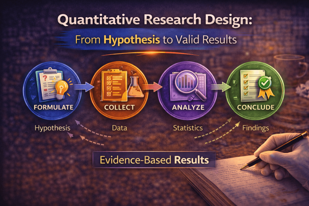
Quantitative Research Design: From Hypothesis to Valid Results
Cluster Post 2 | Module 3: Research Methodologies From Concept to Submission Series | 2026…

Qualitative Research Design: Choosing the Right Approach
Cluster Post 3 | Module 3: Research Methodologies From Concept to Submission Series | 2026…
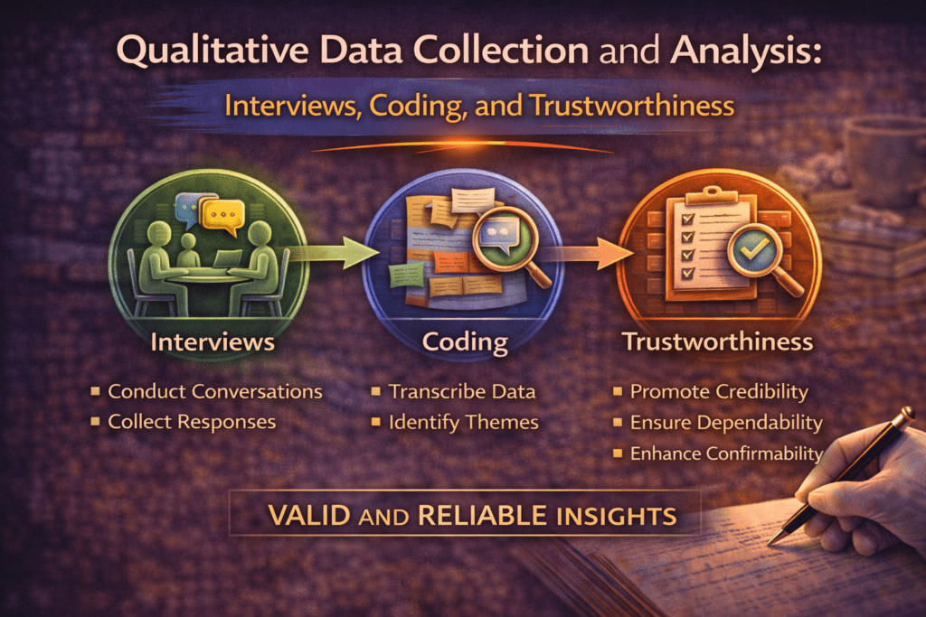
Qualitative Data Collection and Analysis: Interviews, Coding, and Trustworthiness
Cluster Post 4 | Module 3: Research Methodologies From Concept to Submission Series | 2026…
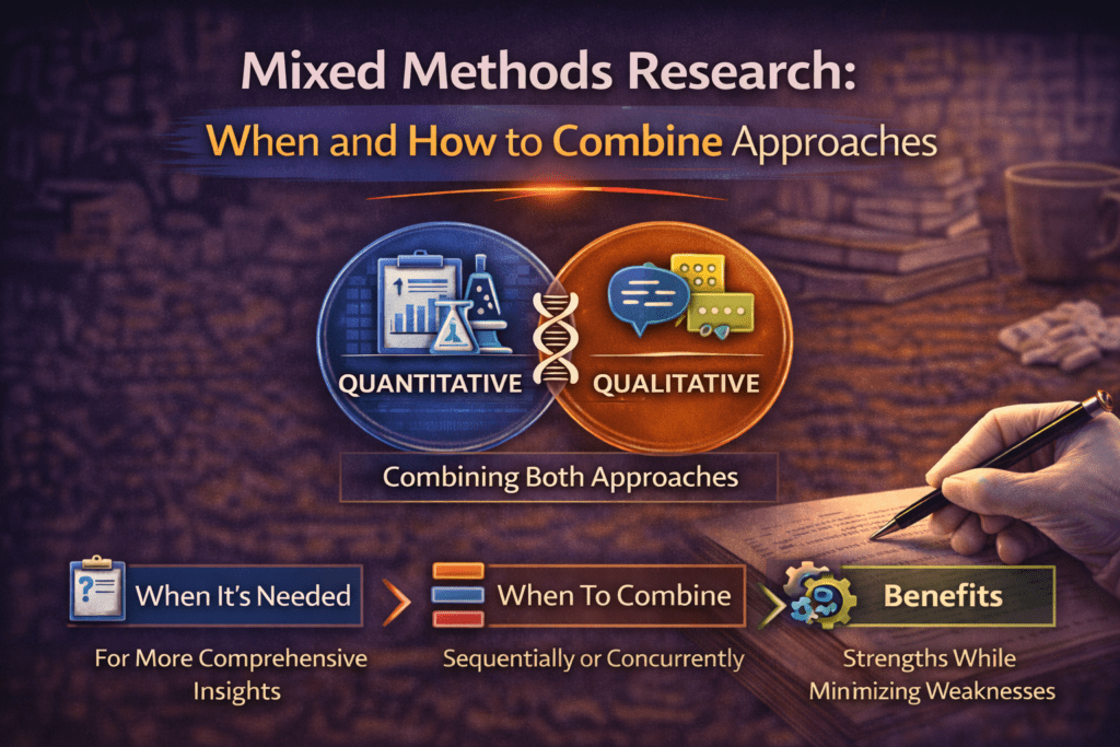
Mixed Methods Research: When and How to Combine Approaches
Cluster Post 5 | Module 3: Research Methodologies From Concept to Submission Series | 2026…
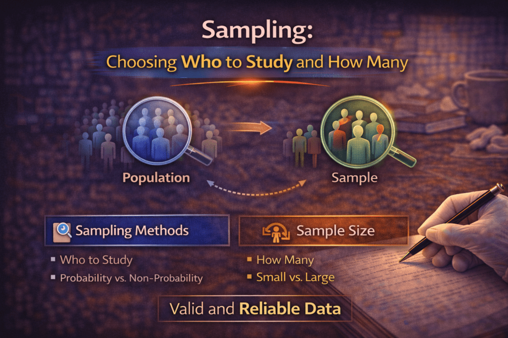
Sampling: Choosing Who to Study and How Many
Cluster Post 6 | Module 3: Research Methodologies From Concept to Submission Series | 2026…

Research Ethics in Practice: What Ethics Forms Don’t Tell You
Cluster Post 7 | Module 3: Research Methodologies From Concept to Submission Series | 2026…
Data Analysis and Results Presentation: Complete Guide for Quantitative, Qualitative & Legal Research (2026)
Data Analysis and Results Presentation: Why Data Analysis Determines Research Credibility Here’s what separates published…
Preparing Your Data: The Work That Determines Analysis Quality
Cluster Post 1 | Module 4: Data Analysis and Presenting Results From Concept to Submission…
Descriptive Statistics: What to Report and How to Read Them
Cluster Post 2 | Module 4: Data Analysis and Presenting Results From Concept to Submission…
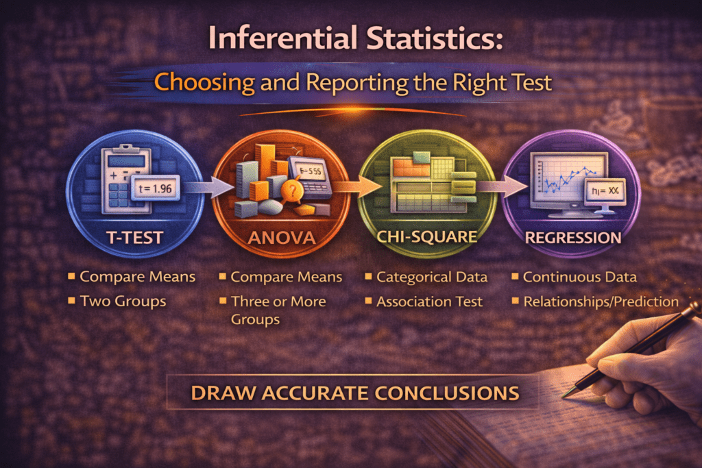
Inferential Statistics: Choosing and Reporting the Right Test
Cluster Post 3 | Module 4: Data Analysis and Presenting Results From Concept to Submission…
Statistical Assumptions: The Checks Most Researchers Skip
Cluster Post 4 | Module 4: Data Analysis and Presenting Results From Concept to Submission…
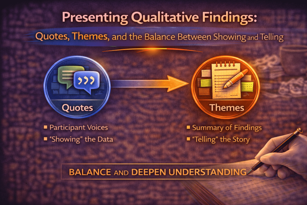
Presenting Qualitative Findings: Quotes, Themes, and the Balance Between Showing and Telling
Cluster Post 5 | Module 4: Data Analysis and Presenting Results From Concept to Submission…
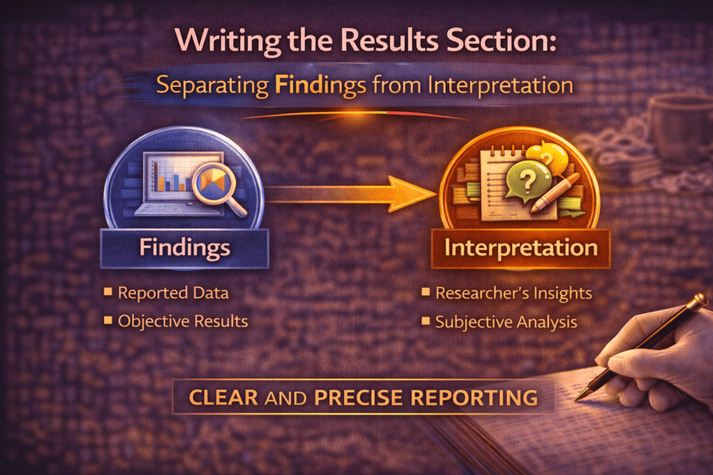
Writing the Results Section: Separating Findings from Interpretation
Cluster Post 6 | Module 4: Data Analysis and Presenting Results From Concept to Submission…

Organization and Academic Tone: Complete Guide to Professional Scholarly Writing (2026)
Why Organization and Academic Tone Matter More Than You Think Here’s what thesis examiners notice…