Last Updated: March 20, 2026
Cluster Post 3 | Module 4: Data Analysis and Presenting Results
From Concept to Submission Series | 2026
Academic Writing Mastery: The Complete 2026 Guide To Research Papers, Thesis & Dissertation Writing
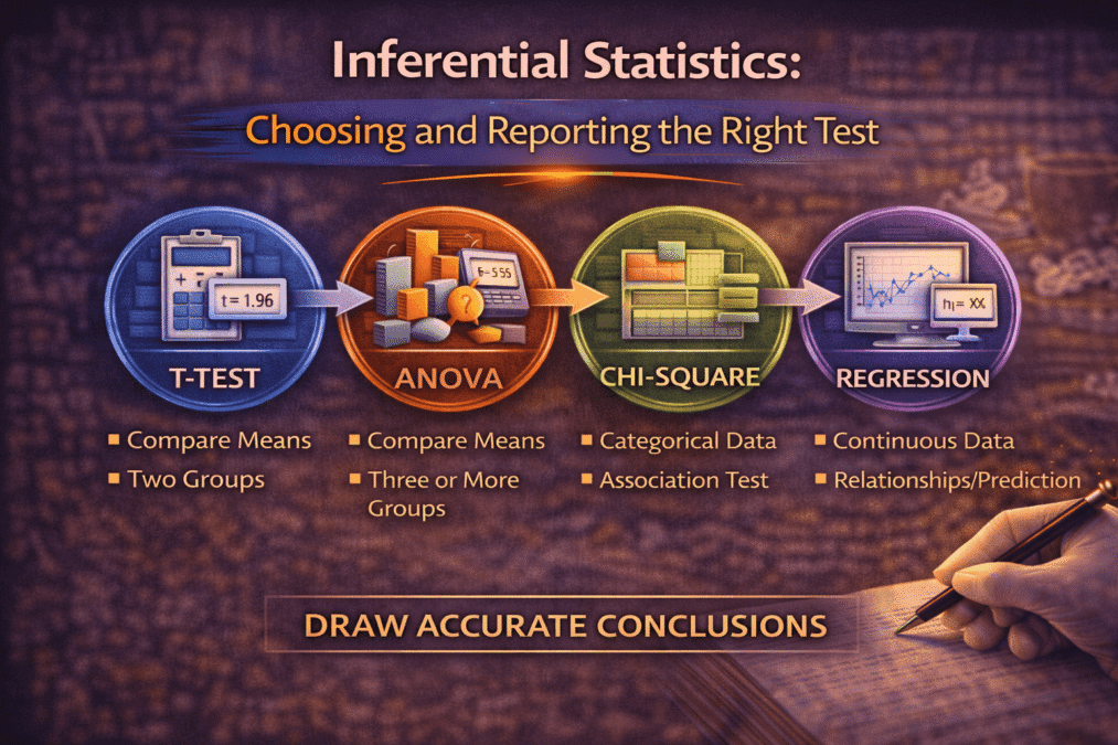
Inferential Statistics: Choosing and Reporting the Right Test

The module overview describes t-tests, ANOVA, correlation, regression, and chi-square. This post goes deeper: a decision framework for choosing the right test, exactly what to report for each test with worked examples, effect sizes explained and why they matter as much as p-values, and the multiple comparisons problem that invalidates many published results.
Choosing the Right Test: The Decision Logic
The most common statistical error in student and early-career research is not running a test incorrectly — it is running the wrong test on the right data. Choosing a test requires answering three questions in sequence: What is the research question asking? What type of variables are involved? Are the assumptions of the candidate test met?
| Research question | Appropriate test |
| Do two independent groups differ on a continuous outcome? | Independent samples t-test (or Mann-Whitney U if normality violated) |
| Does one group differ before vs. after an intervention? | Paired samples t-test (or Wilcoxon signed-rank if normality violated) |
| Do three or more independent groups differ on a continuous outcome? | One-way ANOVA (or Kruskal-Wallis if normality violated) |
| Is there a relationship between two continuous variables? | Pearson correlation (or Spearman’s rho if non-normal) |
| Does one continuous variable predict another? | Simple linear regression |
| Do multiple variables together predict an outcome? | Multiple linear regression |
| Is there a relationship between two categorical variables? | Chi-square test of independence |
| Does a categorical outcome depend on predictors? | Logistic regression |
The non-parametric alternatives in the table — Mann-Whitney U, Wilcoxon, Kruskal-Wallis, Spearman’s rho — are not inferior tests you use when the real test fails. They are the correct tests for data that violates the normality assumption. Using a parametric test on non-normal data with a small sample produces inflated Type I error rates; using the appropriate non-parametric test is the methodologically sound choice.
Understanding p-Values: What They Do and Do Not Tell You
The p-value is the probability of obtaining results at least as extreme as yours if the null hypothesis were true and the study were repeated many times. It is not the probability that the null hypothesis is true. It is not the probability that your findings are a fluke. It is not a measure of the size or importance of an effect.
The .05 threshold is a convention, not a law of nature. Ronald Fisher, who popularised it in the 1920s, described it as a rough guideline for when results were worth further investigation — not as a bright line separating true from false findings. A result with p = .049 is not meaningfully different from one with p = .051. Both represent weak evidence by conventional standards.
Report exact p-values rather than “p < .05” or “n.s.” This allows readers to evaluate the strength of evidence themselves. “p = .043” tells a reader more than “p < .05”. “p = .412” tells a reader more than “n.s.” — particularly when the non-significant result is theoretically informative.
Why effect sizes matter as much as p-values
Statistical significance tells you whether an effect exists. Effect size tells you how large it is. These are different questions, and both matter for interpreting research findings. A study with N = 2,000 will detect very small effects as statistically significant. An effect that is statistically significant but trivially small — d = 0.05, less than one-twentieth of a standard deviation — is not practically meaningful, regardless of its p-value.
Conversely, a study with N = 30 may fail to detect a medium-sized effect as statistically significant simply because it is underpowered. A non-significant result in an underpowered study cannot be interpreted as evidence that the effect does not exist; it is evidence that the study could not detect an effect of the size studied. Effect sizes, combined with confidence intervals, give a more complete picture.
| Effect size measure | Used with | Small / Medium / Large benchmarks |
| Cohen’s d | t-tests: difference between two means | |
| η² (eta-squared) | ANOVA: proportion of variance explained | |
| r | Correlation | |
| R² | Regression: proportion of variance explained by model | |
| Cramér’s V | Chi-square: association between categorical variables |
Reporting Templates for Each Test
APA format specifies exactly what statistical information to include when reporting each test. These are not arbitrary style requirements — they ensure that readers have everything needed to evaluate your results, replicate your analysis, or include your findings in a meta-analysis. The following templates give the required elements.
Independent samples t-test
Students who received peer mentoring (M = 3.74, SD = 0.89) scored significantly higher on the belonging scale than students who did not (M = 3.12, SD = 0.97), t(438) = 7.03, p < .001, d = 0.67. Elements required: group means and SDs, t-statistic, degrees of freedom in parentheses, p-value, effect size (Cohen’s d).
One-way ANOVA
A one-way ANOVA revealed a significant effect of mentoring frequency on belonging scores, F(2, 439) = 14.23, p < .001, η² = .06. Post-hoc comparisons using Tukey’s HSD indicated that students with weekly contact (M = 3.91, SD = 0.84) scored significantly higher than those with monthly contact (M = 3.41, SD = 0.93, p = .003) and those with no contact (M = 3.12, SD = 0.97, p < .001). Monthly and no-contact groups did not differ significantly (p = .21). Elements required: F-statistic, both degrees of freedom (between groups, within groups), p-value, effect size (η²), post-hoc results when overall test is significant.
Pearson correlation
Peer mentor contact frequency was significantly positively correlated with social belonging scores, r(440) = .38, p < .001, 95% CI [.30, .46]. Elements required: r coefficient, N or df in parentheses, p-value, 95% confidence interval. Note: the confidence interval for r is more informative than the p-value alone.
Multiple regression
A multiple regression was conducted to predict social belonging from peer contact frequency, first-generation status, and college type. The model was statistically significant, F(3, 438) = 28.44, p < .001, R² = .16, indicating that the predictors together explained 16% of variance in belonging scores. Peer contact frequency was the strongest predictor (β = .31, p < .001), followed by first-generation status (β = -.18, p = .002). College type was not a significant predictor (β = .07, p = .14). Elements required: overall F and significance, R², standardised coefficients (β) and significance for each predictor. Also report unstandardised B coefficients and standard errors in a table.
Chi-square test of independence
A chi-square test of independence found a significant association between mentoring participation and first-year progression status (pass vs. resit/fail), χ²(1, N = 442) = 12.44, p < .001, Cramér’s V = .17. Elements required: chi-square value, degrees of freedom, N, p-value, effect size (Cramér’s V or phi for 2×2 tables).
The Multiple Comparisons Problem
When you run multiple statistical tests on the same dataset, the probability of obtaining at least one false positive increases substantially. With alpha = .05, you accept a 5% chance of a false positive on any single test. If you run 20 tests, the probability of at least one false positive across all tests rises to approximately 64%.
This is called the familywise error rate, and it inflates silently every time you run more than one test without correction. Many published papers and theses run ten, twenty, or more tests without any correction, which means their “significant” findings may include several that are false positives produced by chance rather than by real effects.
When to apply a correction
Corrections are warranted when you are running multiple tests on the same outcome variable, when you are testing multiple outcomes in an exploratory analysis without strong prior hypotheses, or when individual tests are part of a family of related comparisons (such as all pairwise comparisons in a post-hoc ANOVA test).
The Bonferroni correction is the simplest: divide your alpha level by the number of tests. For 10 tests at alpha = .05, the corrected threshold is .005. It is conservative — it increases the risk of false negatives — but it is straightforward to apply and easy to explain.
For ANOVA post-hoc comparisons, Tukey’s HSD is more powerful than Bonferroni and is the standard recommendation. For complex analyses with many predictors, false discovery rate (FDR) corrections such as the Benjamini-Hochberg procedure offer a less conservative alternative to Bonferroni.
When correction is not required
Corrections are not always necessary. When you have a single, pre-specified primary hypothesis and a small number of secondary hypotheses clearly declared in advance, you can justify testing them without correction — the hypothesis was specified before data collection, so it is not capitalising on chance. The key is transparency: your methodology chapter must clearly distinguish pre-specified primary hypotheses from exploratory analyses, and exploratory analyses require correction.
For Law Students
Quantitative analysis in empirical legal research most commonly uses regression to examine predictors of legal outcomes. Three specific considerations apply in this context.
Logistic regression for binary legal outcomes
Many legal outcomes are binary: case won or lost, bail granted or refused, sentence custodial or non-custodial, appeal upheld or dismissed. Binary outcomes require logistic regression, not linear regression. Linear regression applied to a binary outcome violates assumptions and can produce predicted probabilities outside the 0–1 range — a theoretical and practical impossibility.
Logistic regression reports odds ratios rather than regression coefficients. An odds ratio of 2.3 for the predictor “represented by counsel” means that represented defendants have 2.3 times the odds of a favourable outcome compared to unrepresented defendants, holding other predictors constant. Always report 95% confidence intervals around odds ratios alongside their significance — a wide confidence interval around a large odds ratio signals imprecision that the odds ratio alone does not convey.
Reporting regression results for legal audiences
Legal audiences — including journal reviewers, examiners, and policy audiences — vary widely in statistical literacy. When writing for a primarily legal audience, supplement the statistical reporting with plain-language interpretations of each coefficient. After the formal reporting, add a sentence: “In practical terms, each additional month of case age at the point of listing was associated with a 4.2% increase in the probability of adjournment, controlling for case complexity and court location.” This is not dumbing down — it is translating the statistical finding into terms that allow legal reasoning about its implications.
The ecological fallacy in aggregate court data
When using aggregate court data — statistics at the district or state level rather than the individual case level — be cautious about drawing conclusions about individual cases. If districts with higher caseload show lower grant rates for bail applications, this does not necessarily mean individual judges in high-caseload courts are more likely to refuse bail. The association at district level may be confounded by case composition differences between districts. This is the ecological fallacy — inferring individual-level relationships from aggregate-level correlations — and it requires explicit acknowledgement when aggregate data is used.
FAQs
Q: How do you choose the right statistical test?
Statistical test selection depends on three factors: the research question (relationship, difference, or prediction); the number and type of variables (continuous, categorical, ordinal); and whether the data meets parametric assumptions (normality, homogeneity of variance). For comparing two groups on a continuous variable: independent t-test (parametric) or Mann-Whitney U (non-parametric). For comparing three or more groups: ANOVA or Kruskal-Wallis. For relationships between continuous variables: Pearson correlation or Spearman’s rho. For predicting a continuous outcome: regression. For categorical outcomes: chi-square or logistic regression.
Q: What is a p-value and how do you interpret it?
A p-value is the probability of obtaining results at least as extreme as the observed results, assuming the null hypothesis is true. A p-value of 0.05 means there is a 5% probability the results occurred by chance if the null hypothesis is correct. The conventional threshold is p < 0.05 for statistical significance. A p-value does not tell you the size or practical importance of an effect — a very small effect can be statistically significant with a large sample. Always report effect size alongside p-values. Never report p = 0.000 — use p < .001.
Q: What is effect size and why does it matter?
Effect size quantifies the practical magnitude of a finding, independent of sample size. A statistically significant result with a tiny effect size may be meaningless in practice; a non-significant result with a large effect size may be practically important but underpowered. Common effect size measures: Cohen’s d for t-tests (small = 0.2, medium = 0.5, large = 0.8); eta-squared (η²) for ANOVA; r for correlations; odds ratios for logistic regression. Most journals now require effect size reporting — p-values alone are insufficient.
Q: What is the difference between correlation and causation in research?
Correlation means two variables are statistically associated — when one changes, the other tends to change. Causation means one variable directly produces change in another. Correlation does not imply causation. To establish causation, you need: temporal precedence (cause precedes effect); covariation (the two are correlated); and elimination of alternative explanations (achieved through experimental control or statistical techniques like regression with covariates). Cross-sectional surveys establish correlation only. Experimental and longitudinal designs can establish causation under specific conditions.
Q: What is regression analysis and when do you use it?
Regression analysis examines the relationship between a dependent variable and one or more independent variables, while controlling for other variables simultaneously. Linear regression predicts a continuous outcome (exam scores, income). Logistic regression predicts a binary outcome (pass/fail, employed/unemployed). Multiple regression allows you to identify which predictors are independently associated with the outcome after controlling for others. Report: the regression coefficient (B), standardised coefficient (β), p-value, and R² (variance explained) for each predictor. Always check and report whether regression assumptions are met.
References
- Field, A. (2024). Discovering Statistics Using IBM SPSS Statistics (6th ed.). Sage.
- Cohen, J. (1988). Statistical Power Analysis for the Behavioral Sciences (2nd ed.). Lawrence Erlbaum.
- Cumming, G. (2014). The new statistics: Why and how. Psychological Science, 25(1), 7–29.
- American Psychological Association. (2020). Publication Manual of the APA (7th ed.).
- Tabachnick, B. G., & Fidell, L. S. (2022). Using Multivariate Statistics (8th ed.). Pearson.
- Frost, J. (2023). Regression Analysis: An Intuitive Guide. Statistics By Jim Publishing.
Next: Cluster Post 4 — Statistical Assumptions: The Checks Most Researchers Skip
Module 1 (Pillar Post)- The Complete Guide To Research Paper Structure: IMRAD Format, Thesis Organization & Academic Writing (2026)
Module 2 (Pillar Post) –The Academic Writing Process: Complete Guide from First Draft to Submission (2026)
Module 3 (Pillar Post): Research Methodologies: Complete Guide to Quantitative, Qualitative, Mixed Methods & Legal Research (2026)
- Pillar Post : Organization and Academic Tone: Complete Guide to Professional Scholarly Writing (2026) (Module 5)
- Pillar Post : Peer Review and Publication: Complete Guide from Submission to Acceptance (2026) (Module 6)
- Pillar Post : AI Tools in Academic Research: Opportunities, Ethics, and Best Practices (2026) (Module 7)
- Pillar Post: Grant Writing and Research Funding: Complete Guide to Finding Money for Your Research (2026) (Module 8)
- Pillar Post : Academic Career Development: Complete Guide to Building Your Professional Life in Research (2026) (Module 9)
- Pillar Post : Research Ethics and the IRB Process: Complete Guide to Doing Research Responsibly (2026) (Module 10)

The Complete Guide to Research Paper Structure: IMRAD Format, Thesis Organization & Academic Writing (2026)
From Concept to Submission: A Complete Guide to Research Paper and Thesis Writing Academic Writing…
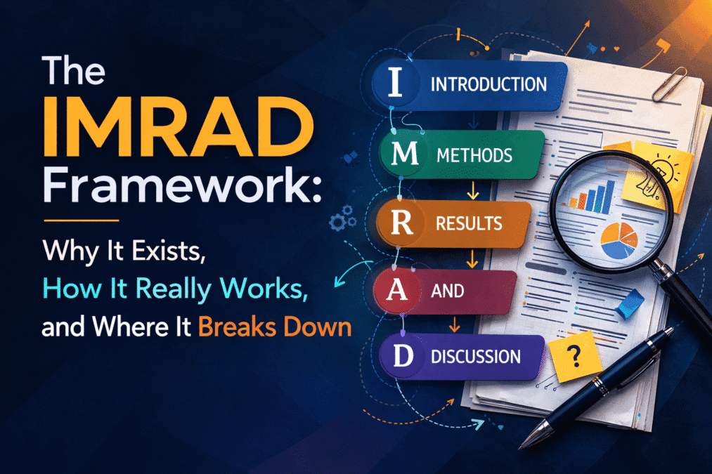
The IMRAD Framework: Why It Exists, How It Really Works, and Where It Breaks Down
The IMRAD Framework Understanding the Structure of Research Papers and Theses – Module 1: From Concept…

How to Write a Research Introduction That Reviewers Cannot Ignore
How to Write a Research Introduction Module 1: Understanding the Structure of Research Papers and…

How to Write a Methods Section That Reviewers Will Trust
How to Write a Methods Section Module 1: Understanding the Structure of Research Papers and…
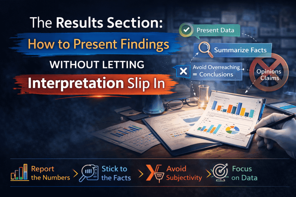
The Results Section: How to Present Findings Without Letting Interpretation Slip In
The Results Section Module 1: Understanding the Structure of Research Papers and Theses From Concept…

The Discussion Section: How to Turn Findings Into Knowledge
The Discussion Section Module 1: Understanding the Structure of Research Papers and Theses From Concept…

Complete Thesis Structure: A Chapter-by-Chapter Guide
Complete Thesis Structure Module 1: Understanding the Structure of Research Papers and Theses From Concept…

10 Structural Mistakes That Get Research Papers Rejected — And How to Fix Every One
10 Structural Mistakes That Get Research Papers Rejected Module 1: Understanding the Structure of Research…

How to Write a Journal Abstract That Gets Your Paper Read
How to Write a Journal Abstract Module 1: Understanding the Structure of Research Papers and…
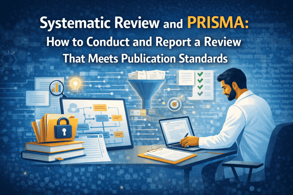
Systematic Review and PRISMA: How to Conduct and Report a Review That Meets Publication Standards
Systematic Review and PRISMA Module 1: Understanding the Structure of Research Papers and Theses From…

Legal Research Methods: A Complete Guide to Doctrinal, Empirical and Comparative Legal Research
Legal Research Methods Module 1: Understanding the Structure of Research Papers and Theses From Concept…

The Academic Writing Process: Complete Guide from First Draft to Submission (2026)
Module 2, Complete Guide: The Academic Writing Process – from First Draft to Submission From…

How to Start Writing and Keep Going
How to Start Writing Module 2: The Academic Writing Process From Concept to Submission Series …

How to Write Clear Engaging Academic Prose
How to Write Clear Engaging Academic Prose – Module 2: The Academic Writing Process From…

The Revision Process: How to Turn a Draft Into a Submission
The Revision Process Module 2: The Academic Writing Process From Concept to Submission Series | …

Citation Styles Explained: APA, MLA, Chicago, IEEE, and Bluebook
Citation Styles Explained Module 2: The Academic Writing Process From Concept to Submission Series | …

Preparing a Submission Ready Document: The Complete Pre-Submission Checklist
Preparing a Submission Ready Document Module 2: The Academic Writing Process From Concept to Submission…

Reference Management: Zotero and Mendeley from Setup to Submission
Reference Management Module 2: The Academic Writing Process From Concept to Submission Series | 2026 Academic…

Legal Writing Process and Citation: A Complete Guide for Law Students and Legal Researchers
Legal Writing Process and Citation Module 2: The Academic Writing Process From Concept to Submission…

Research Methodologies: Complete Guide to Quantitative, Qualitative & Mixed Methods (2026)
(Module 3) – Complete Guide Research Methodologies From Concept to Submission: A Complete Guide to…

Research Paradigms: Why Your Philosophical Stance Shapes Everything
Research Paradigms Module 3: Research Methodologies From Concept to Submission Series | 2026 Academic Writing Mastery:…
Quantitative Research Design: From Hypothesis to Valid Results
Quantitative Research Design Module 3: Research Methodologies From Concept to Submission Series | 2026 Academic…

Qualitative Research Design: Choosing the Right Approach
Qualitative Research Design Module 3: Research Methodologies From Concept to Submission Series | 2026 Academic…
Qualitative Data Collection and Analysis: Interviews, Coding, and Trustworthiness
Qualitative Data Collection and Analysis Module 3: Research Methodologies From Concept to Submission Series | …
Mixed Methods Research: When and How to Combine Approaches
Mixed Methods Research Module 3: Research Methodologies From Concept to Submission Series | 2026 Academic…
Sampling: Choosing Who to Study and How Many
Sampling Module 3: Research Methodologies From Concept to Submission Series | 2026 Academic Writing Mastery:…

Research Ethics in Practice: What Ethics Forms Don’t Tell You
Research Ethics in Practice Module 3: Research Methodologies From Concept to Submission Series | 2026…
Data Analysis and Results Presentation: Complete Guide for Quantitative & Qualitative Research (2026)
(Module 4) Data Analysis and Results Presentation: From Concept to Submission: A Complete Guide to…

Preparing Your Data: The Work That Determines Analysis Quality
Cluster Post 1 | Module 4: Data Analysis and Presenting Results From Concept to Submission…
Descriptive Statistics: What to Report and How to Read Them
Cluster Post 2 | Module 4: Data Analysis and Presenting Results From Concept to Submission…